


TurboQuant is a vector quantization algorithm from Google Research (ICLR 2026, arXiv:2504.19874) that compresses LLM key-value caches to roughly 3 bits per coordinate with zero accuracy loss. It combines PolarQuant — a rotation-based coordinate transform — with a 1-bit QJL residual correction, achieving at least 6× memory reduction and up to 8× faster attention computation on NVIDIA H100 GPUs. The method is data-oblivious, requires no training, and operates within a factor of ≈2.7 of the information-theoretic limit.
Why Does KV Cache Size Limit LLM Inference?
Every time a decoder-based transformer generates a new token, it stores a key vector and a value vector for that token in every attention layer. This collection of vectors — the key-value (KV) cache — is the model’s working memory for the current context.
The problem is straightforward: KV cache size scales linearly with both model depth (number of layers × attention heads) and context length. A model like Qwen2.5-3B with 36 layers accumulates roughly 289 MB of KV cache at 8K tokens in FP16 precision. On a 12 GB consumer GPU, the KV cache — not the model weights — becomes the binding constraint on how long a context the model can process. At 128K tokens, production models like Llama-3.1-8B-Instruct can consume over 4 GB of KV cache in FP16, forcing engineers to choose between context length and batch size.
Quantization compresses these vectors from 16-bit floats to lower precision (4-bit, 3-bit, or even 2-bit integers), reducing memory proportionally. But naïve scalar quantization at very low bit-widths destroys the geometric relationships between vectors — specifically, their inner products (dot products) — which are exactly what the attention mechanism computes. This is where TurboQuant enters the picture.
The KV cache memory formula
It helps to see the exact arithmetic, because it shows precisely where a bit-width reduction lands. The KV cache size for a single sequence is:
KV bytes = 2 × layers × kv_heads × head_dim × seq_len × bytes_per_value
The leading 2 covers one key plus one value per token. kv_heads is the number of key/value heads (with grouped-query attention this is far smaller than the number of query heads). bytes_per_value is 2 for FP16 and 0.375 for 3-bit TurboQuant (3 bits ÷ 8).
Worked example, Llama-3.1-8B-Instruct (32 layers, 8 KV heads, head_dim 128) at a 128K context, batch size 1:
| Precision | Bytes/value | KV cache @ 128K | vs FP16 |
|---|---|---|---|
| FP16 (baseline) | 2.0 | ≈ 16 GB | 1× |
| 4-bit | 0.5 | ≈ 4 GB | 4× |
| 3-bit TurboQuant | 0.375 | ≈ 3 GB | ≈ 5.3× |
The same model with multi-head attention (no GQA) would be 4× larger again — which is exactly why memory-bound inference moved to grouped-query attention and aggressive KV quantization at the same time. TurboQuant attacks the second lever.
What Is TurboQuant and How Does It Work?
TurboQuant is a two-stage vector quantization algorithm designed by researchers at Google Research and New York University. It was published at ICLR 2026 (originally posted as arXiv:2504.19874 in April 2025) and builds on two companion papers: PolarQuant (AISTATS 2026) and Quantized Johnson-Lindenstrauss / QJL.
The core insight is that MSE-optimal quantizers introduce systematic bias in inner product estimation. TurboQuant solves this by splitting the compression budget into two stages:
Stage 1: PolarQuant — MSE-Optimal Compression
The input vector is multiplied by a random orthogonal matrix (generated via QR decomposition of a Gaussian matrix). This rotation has a critical mathematical effect: after rotation, each coordinate follows a concentrated Beta distribution — well-approximated by Gaussian N(0, 1/d) for typical head dimensions. Because this distribution is known and coordinates become nearly independent in high dimensions, you can apply an optimal Lloyd-Max scalar quantizer to each coordinate independently.
Lloyd-Max quantization solves a continuous k-means problem: given a known distribution and a bit budget (e.g., 3 bits = 8 reconstruction levels), it finds the bucket boundaries and centroids that minimize mean squared error. The codebooks are precomputed once per bit-width — they do not depend on the data at all. This is what makes TurboQuant data-oblivious and suitable for online (streaming) applications like KV cache compression, where vectors arrive one token at a time.
Traditional methods (e.g., per-channel min-max quantization) need to store normalization constants (scale and zero-point) for every small block of data — typically adding 1–2 extra bits per coordinate of overhead. PolarQuant eliminates this overhead entirely because the post-rotation distribution is fixed and known in advance.
Stage 2: QJL — 1-Bit Residual Correction
Stage 1 minimizes MSE but introduces a small bias in dot products. For the attention mechanism, which computes Q·K dot products to produce attention scores, this bias accumulates across tokens.
TurboQuant corrects this by applying the Quantized Johnson-Lindenstrauss (QJL) transform to the residual vector (the difference between the original and quantized vector). QJL reduces each coordinate of the residual to a single sign bit (+1 or −1), adding exactly 1 bit per coordinate of overhead with zero additional memory for normalization constants. The resulting combined estimator for the inner product is provably unbiased.
The total bit-width is therefore (b − 1) bits for PolarQuant + 1 bit for QJL = b bits total. At 3 bits total, the method achieves what the paper calls “absolute quality neutrality” — no measurable accuracy degradation compared to FP16.
What Do the Benchmarks Show?
Google Research evaluated TurboQuant across multiple long-context benchmarks — LongBench, Needle-In-A-Haystack, ZeroSCROLLS, RULER, and L-Eval — using open-source models (Gemma, Mistral, Llama-3.1-8B-Instruct). The results are striking:
| Metric | 3-bit TurboQuant | 4-bit TurboQuant | FP16 Baseline |
|---|---|---|---|
| LongBench aggregate score | Quality neutral | Quality neutral | 100% |
| Needle-In-A-Haystack | Perfect retrieval | Perfect retrieval | Perfect retrieval |
| KV memory reduction | ≥ 6× | ≥ 4× | 1× |
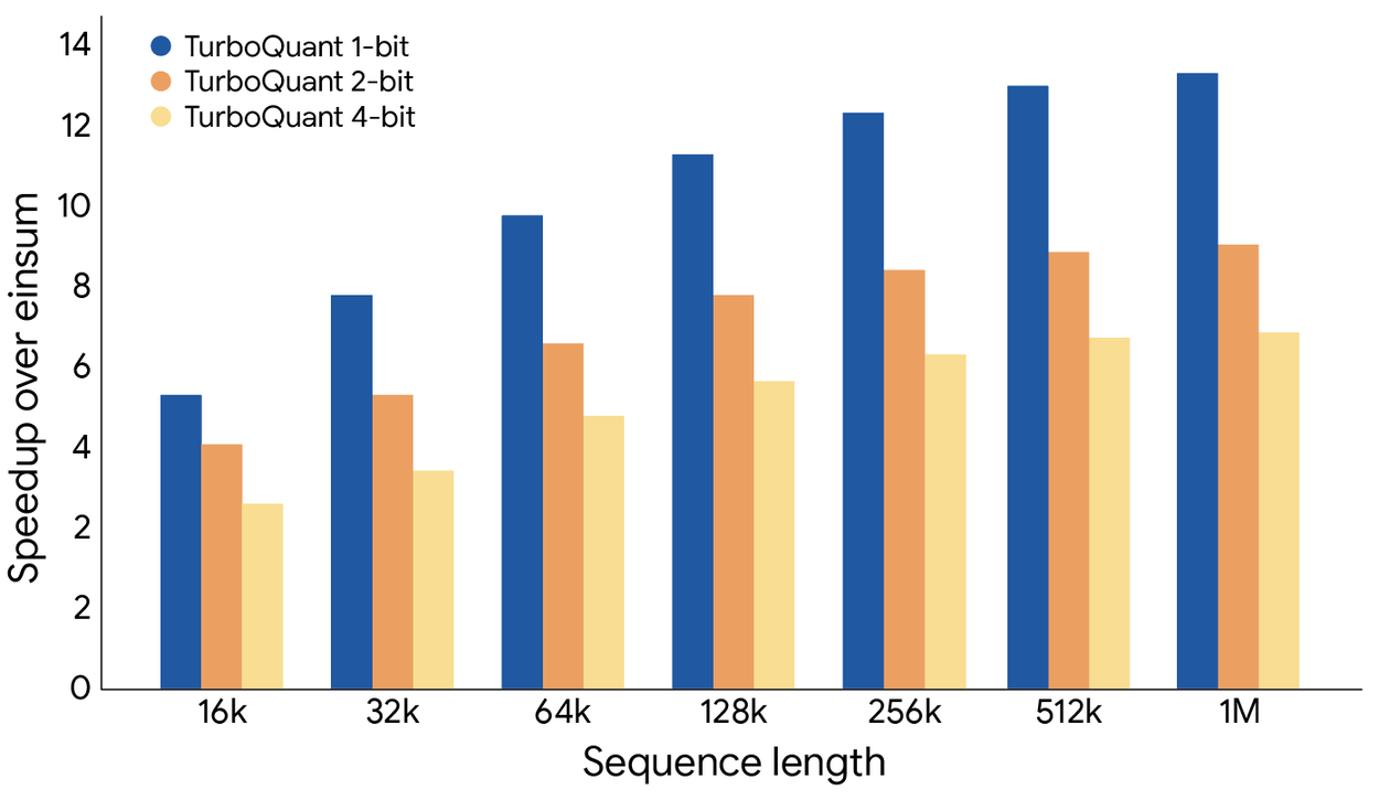
| Attention speedup (H100) | — | Up to 8× | 1× |
| Training / fine-tuning required | None | None | — |
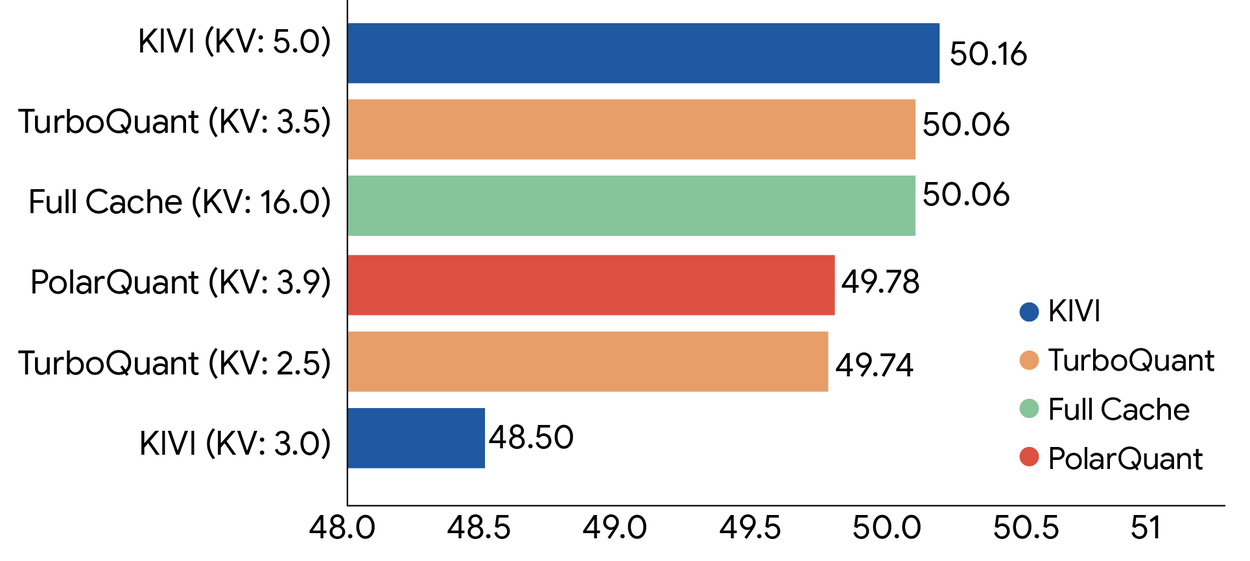
Community reimplementations confirm the paper’s claims. A from-scratch PyTorch implementation tested on Qwen2.5-3B-Instruct reports 99.5% cosine similarity between compressed and original attention scores at 3-bit, with 9/9 exact nearest-vector retrieval across all bit-widths and context lengths tested. At 3 bits, the KV cache for an 8K-token context drops from 289 MB to 58 MB — the difference between fitting ~8K context and ~40K context on a 12 GB GPU.
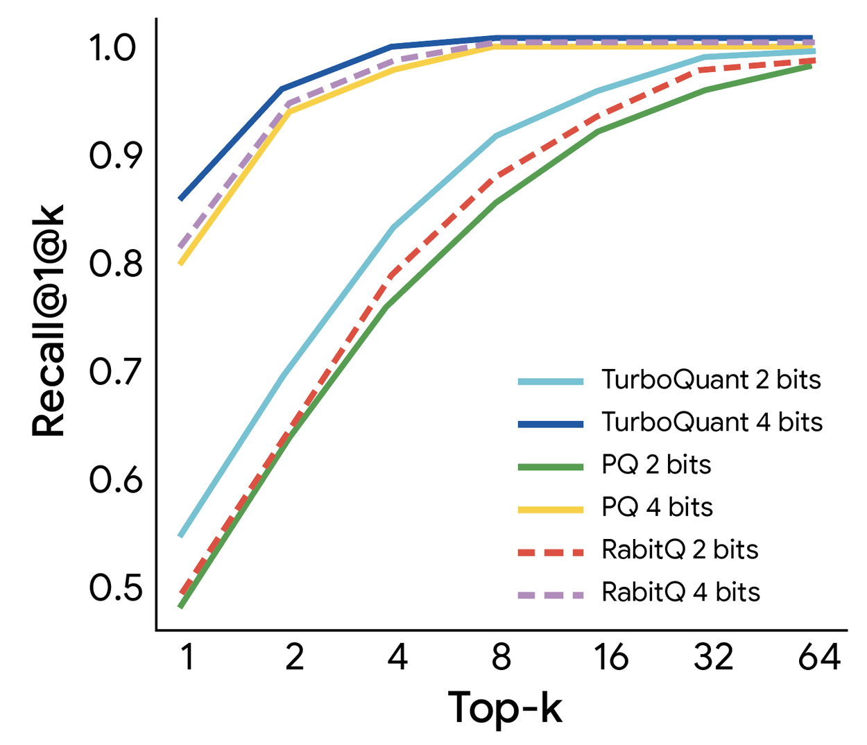
For nearest neighbor search on the GloVe embedding dataset (d=200), TurboQuant achieved the best recall ratios across top-k retrieval tasks compared to standard Product Quantization and RaBitQ, while reducing indexing time to virtually zero (because codebooks are precomputed, not learned from data).
How Does TurboQuant Compare to Other KV Cache Compression Methods?
The KV cache compression landscape has evolved rapidly. Here is where TurboQuant sits relative to key alternatives:
| Method | Type | Min bits | Training needed | Inner product unbiased |
|---|---|---|---|---|
| TurboQuant (ICLR 2026) | Data-oblivious VQ | 2.5–3 | No | Yes (with QJL) |
| KIVI | Per-channel scalar | 2 | No | No |
| KVQuant (NeurIPS 2024) | NUQ + dense-sparse | 3 | Calibration | No |
| CommVQ (ICML 2025) | Additive VQ + codebook | 2 | EM training | No |
| VQKV (2026) | SimVQ + residual codebooks | ~1 (index) | No (training-free) | No |
| VecInfer (2025) | Hadamard + VQ | 2 | No | No |
TurboQuant’s distinctive properties are the combination of provable near-optimality (within ≈2.7× of Shannon’s distortion-rate bound), unbiased inner product estimation, zero training requirements, and zero normalization overhead. Most competing methods either require calibration data, store per-block normalization constants that add 1–2 bits of overhead, or both.
An expert analysis notes that most easy compression gains (2–3× from basic int8/int4 quantization, 3–4× with outlier-aware methods like SmoothQuant/AWQ) are already deployed in production LLM systems. TurboQuant pushes the boundary to approximately 4–4.5× effective compression. The remaining gains are real but smaller, and each additional step is increasingly expensive to implement and stabilize in production. The theory is settled — the engineering challenge is the bottleneck.
TurboQuant, QJL, PolarQuant and RotorQuant: the method family
TurboQuant did not appear in isolation — it is the convergence point of a short lineage of papers from the same research group. If you have seen these names searched together, here is how they actually relate:
| Method | arXiv / venue | Role in the family |
|---|---|---|
| QJL (Quantized Johnson-Lindenstrauss) | 2406.03482 | The 1-bit, zero-overhead sign-quantization transform with an unbiased inner-product estimator. It is the residual-correction stage TurboQuant reuses in Stage 2. |
| PolarQuant | 2502.02617 · AISTATS 2026 | The rotation + polar-coordinate transform that makes the post-rotation distribution known and concentrated, removing per-block normalization overhead. It is TurboQuant’s Stage 1. |
| TurboQuant | 2504.19874 · ICLR 2026 | The unification: PolarQuant (MSE-optimal) + QJL (1-bit residual) → a single data-oblivious quantizer that is both MSE-optimal and unbiased on inner products, within ≈2.7× of the Shannon distortion-rate bound. |
| RotorQuant (community variant) | open-source | A Clifford-algebra reformulation of TurboQuant with fused Triton kernels; community benchmarks claim 10–19× faster quantization with far fewer parameters at large d. Not an official Google paper. |
The mental model: QJL solved the unbiased-inner-product problem, PolarQuant solved the normalization-overhead problem, and TurboQuant fuses both into one online algorithm with a formal optimality proof. When people search “TurboQuant PolarQuant QJL paper” or “quantized Johnson-Lindenstrauss,” they are usually trying to reconstruct exactly this lineage — the canonical reference is arXiv 2504.19874.
What Does the Math Actually Guarantee?
TurboQuant comes with formal information-theoretic proofs. The paper derives Shannon lower bounds on the best achievable distortion rate for any vector quantizer and shows that TurboQuant’s distortion differs from these bounds by only a constant factor of approximately 2.7. This is significant: it means no algorithm — regardless of computational cost or data dependence — can fundamentally do more than ~2.7× better than TurboQuant at the same bit budget.
Formally, for a b-bit quantizer operating on unit-norm vectors in ℝᵈ, TurboQuant achieves MSE distortion proportional to 2⁻²ᵇ, which matches the exponential scaling of the Shannon bound. The factor of 2.7 comes from the gap between the Lloyd-Max quantizer (which is optimal for scalar quantization of a known distribution) and the theoretical limit for vector quantization of the same distribution.
For practitioners, the implication is straightforward: at 3.5 bits per coordinate, TurboQuant achieves “absolute quality neutrality” (zero measurable degradation). At 2.5 bits, degradation is marginal. Going below 2 bits per coordinate, any method — including TurboQuant — will hit the information-theoretic wall.
How Can You Use TurboQuant Today?
As of mid-2026, TurboQuant is not yet integrated into mainstream inference frameworks (vLLM, TGI, llama.cpp), but several open-source implementations exist:
import torch
import numpy as np

# Stage 1: Random rotation (PolarQuant)
def random_rotation_matrix(d: int) -> torch.Tensor:
    """Generate random orthogonal matrix via QR decomposition."""
    G = torch.randn(d, d)
    Q, R = torch.linalg.qr(G)
    # Ensure proper orthogonal matrix (det = +1)
    Q *= torch.sign(torch.diag(R))
    return Q

# Lloyd-Max codebooks are precomputed for Beta distribution
# Example for 3-bit (8 levels), d=128
CODEBOOK_3BIT = precompute_lloyd_max(n_levels=8, d=128)

def turboquant_encode(x: torch.Tensor, R: torch.Tensor,
                      codebook: dict, n_bits: int = 3):
    """Encode vector x using TurboQuant two-stage pipeline."""
    norm = x.norm()
    x_unit = x / norm

    # Stage 1: Rotate and scalar-quantize
    x_rot = R @ x_unit
    indices = quantize_lloyd_max(x_rot, codebook)
    x_recon = dequantize_lloyd_max(indices, codebook)

    # Stage 2: QJL on residual
    residual = x_rot - x_recon
    qjl_bits = torch.sign(residual)  # 1-bit per coord

    return norm, indices, qjl_bits

def turboquant_decode(norm, indices, qjl_bits,
                      R: torch.Tensor, codebook: dict):
    """Decode: reconstruct approximate vector."""
    x_recon = dequantize_lloyd_max(indices, codebook)
    # QJL correction for unbiased inner products
    x_corrected = x_recon  # + qjl_correction_term
    x_orig_space = R.T @ x_corrected
    return norm * x_orig_space
Production-quality implementations are available on GitHub — notably tonbistudio/turboquant-pytorch (validated on Qwen2.5-3B, RTX 3060) and scrya-com/rotorquant (a Clifford algebra variant with Triton GPU kernels, benchmarked on RTX 5090). The RotorQuant variant claims 10–19× faster quantization than the reference TurboQuant with 44× fewer parameters at d=4096.
What Does This Mean for RAG and Vector Search?
TurboQuant is not limited to KV cache compression. The same algorithm applies directly to vector databases used in retrieval-augmented generation (RAG) and nearest neighbor search. Traditional Product Quantization (PQ) for vector search requires expensive offline training — clustering the dataset to build codebooks that are specific to the data distribution. TurboQuant’s codebooks are data-oblivious and precomputed, meaning indexing time drops to virtually zero while recall either matches or exceeds PQ on standard benchmarks. If you are choosing a store for these vectors, see our guide to vector databases.
For RAG pipelines where the embedding database changes frequently (new documents added, old ones removed), the elimination of codebook retraining is a significant operational advantage. The vectors can be quantized as they arrive — no batch processing, no reindexing.
What Does This Mean in Practice?
For engineers running LLM inference:
The immediate practical impact is straightforward: at 3-bit quantization, a model that previously needed 4 GB of KV cache for a 128K context can run in under 700 MB. On a single A100 80 GB or H100 GPU, this translates directly to either longer contexts or larger batch sizes — both of which reduce per-token cost. The absence of any training or calibration step means TurboQuant can be dropped into existing inference pipelines without reprocessing the model. The same memory math drives the economics of hosted inference — see how providers price it in our best inference APIs comparison.
The deeper significance is that TurboQuant marks the point where KV cache compression is approaching a hard information-theoretic boundary. The ≈2.7× gap to the Shannon bound leaves limited room for future improvement. Most future gains in LLM memory efficiency will need to come from architectural changes (e.g., multi-query attention, shared KV heads, sliding window attention) rather than better compression of the same data.
For the LLM ecosystem broadly, TurboQuant — together with methods like KVQuant, CommVQ, and VQKV — is closing the gap between what the theory allows and what deployed systems achieve. The compression question is increasingly solved; the remaining challenges are kernel-level GPU implementation and integration into inference frameworks.
FAQ
Bibliography
Zandieh, A., Daliri, M., Hadian, M., & Mirrokni, V. (2025). TurboQuant: Online Vector Quantization with Near-optimal Distortion Rate. ICLR 2026. https://arxiv.org/abs/2504.19874
Zandieh, A., Han, I., Daliri, M., & Karbasi, A. (2024). QJL: 1-Bit Quantized JL Transform for KV Cache Quantization with Zero Overhead. https://arxiv.org/abs/2406.03482
Zandieh, A., Hadian, M., & Mirrokni, V. (2025). PolarQuant: Quantizing KV Caches with Polar Transformation. AISTATS 2026. https://arxiv.org/abs/2502.02617
Google Research. (2026, March 24). TurboQuant: Redefining AI efficiency with extreme compression. Google Research Blog. https://research.google/blog/turboquant-redefining-ai-efficiency-with-extreme-compression/
Hooper, C., Kim, S., Mohammadzadeh, H., Mahoney, M. W., Shao, Y. S., Keutzer, K., & Gholami, A. (2024). KVQuant: Towards 10 Million Context Length LLM Inference with KV Cache Quantization. NeurIPS 2024. https://arxiv.org/abs/2401.18079
Vaswani, A., Shazeer, N., Parmar, N., et al. (2017). Attention Is All You Need. NeurIPS 2017, 5998–6008. https://arxiv.org/abs/1706.03762
Shannon, C. E. (1959). Coding theorems for a discrete source with a fidelity criterion. IRE National Convention Record, 7(4), 142–163.